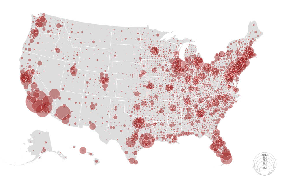
Geographical Map

1. Load data

This example has the dependency pytopojson which has some bugs that I fixed on a fork. The author of pytopojson is busy and does not have the time to update pytopojson unfortunately.

You must install a fork of pytopojson by running this command:

pip install git+https://github.com/bourbonut/pytopojson.git

# https://observablehq.com/@d3/bubble-map/2
import detroit as d3
import requests
import json
from pytopojson.feature import Feature
from pytopojson.mesh import Mesh
from math import isnan

URL = (
    "https://static.observableusercontent.com/files/beb56a2d9534662123fa352ffff2db8472e"
    "481776fcc1608ee4adbd532ea9ccf2f1decc004d57adc76735478ee68c0fd18931ba01fc859ee4901d"
    "eb1bee2ed1b?response-content-disposition=attachment%3Bfilename*%3DUTF-8%27%27popul"
    "ation.json"
)
US_URL = "https://cdn.jsdelivr.net/npm/us-atlas@3/counties-10m.json"

# Load data
population = json.loads(requests.get(URL).content)
us = json.loads(requests.get(US_URL).content)
nation = Feature()(us, us["objects"]["nation"])
statemap = dict(
    (d["id"], d) for d in Feature()(us, us["objects"]["states"])["features"]
)
countymap = dict(
    (d["id"], d) for d in Feature()(us, us["objects"]["counties"])["features"]
)
statemesh = Mesh()(
    us,
    obj=us["objects"]["states"],
    filt=lambda a, b: a != b,
)
countymesh = Mesh()(
    us,
    obj=us["objects"]["counties"],
    filt=lambda a, b: a != b and int(int(a["id"]) / 1000) == int(int(b["id"]) / 1000),
)

# Declare the chart dimensions.
width = 975
height = 610

projection = (
    d3.geo_albers_usa().scale(width * 1.2).translate([width * 0.5, height * 0.5])
)


# Helps to compute centroid positions
class Centroid:
    def __init__(self):
        self._centroid = d3.geo_path(projection).centroid

    def __call__(self, feature):
        return f"translate({','.join(map(str, self._centroid(feature)))})"

    def is_valid(self, feature):
        return not any(map(isnan, self._centroid(feature)))


centroid = Centroid()

# Process data
population = [
    {
        "state": statemap.get(state),
        "county": countymap.get(f"{state}{county}"),
        "fips": f"{state}{county}",
        "population": int(p),
    }
    for p, state, county in population[1:]
]
data = sorted(
    filter(lambda d: centroid.is_valid(d["county"]), population),
    key=lambda d: d["population"],
    reverse=True,
)

2. Make the map

# Declare the radius scale.
radius = d3.scale_sqrt([0, data[0]["population"]], [0, 40])
path = d3.geo_path(projection)

# Create the SVG container.
svg = (
    d3.create("svg")
    .attr("width", width)
    .attr("height", height)
    .attr("viewBox", f"0 0 {width} {height}")
    .attr("style", "width:100%;height:auto;")
)

# Append US nations
svg.append("path").datum(nation).attr("fill", "#ddd").attr("d", path)

# Append borderlands of states
(
    svg.append("path")
    .datum(statemesh)
    .attr("fill", "none")
    .attr("stroke", "white")
    .attr("stroke-linejoin", "round")
    .attr("d", path)
)

# Append legend
legend = (
    svg.append("g")
    .attr("fill", "#777")
    .attr("transform", "translate(915,608)")
    .attr("text-anchor", "middle")
    .style("font", "10px sans-serif")
    .select_all()
    .data(radius.ticks(4)[1:])
    .join("g")
)

# Append circles in legend
(
    legend.append("circle")
    .attr("fill", "none")
    .attr("stroke", "#ccc")
    .attr("cy", lambda d: -radius(d))
    .attr("r", radius)
)

# Append texts in legend
(
    legend.append("text")
    .attr("y", lambda d: -2 * radius(d))
    .attr("dy", "1.3em")
    .text(radius.tick_format(4, "s"))
)

# Append red circles and description when the mouse overs a red circle (only
# available on SVG)
formatter = d3.format(",.0f")
(
    svg.append("g")
    .attr("fill", "brown")
    .attr("fill-opacity", 0.5)
    .attr("stroke", "white")
    .attr("stroke-width", 0.5)
    .select_all()
    .data(data)
    .join("circle")
    .attr("transform", lambda d: centroid(d["county"]))
    .attr("r", lambda d: radius(d['population']))
    .append("title")
    .text(lambda d: f"{d['county']['properties']['name']}, {d['state']['properties']['name']} {formatter(d['population'])}")
)

3. Save your chart

with open("bubble-map.svg", "w") as file:
    file.write(str(svg))